New York City Taxi and Limousine Commission (TLC) Trip Record Data Analysis
Motivation
You’ll know which city I am talking about if I start describing it as the most populous city in the States, one of the biggest and the best places to be, the Big Apple, The City that never sleeps (literally). You got it right! Its NYC! I am very sure, that out of the many things that pop in your mind when you think of New York, the yellow taxicab 🚖 definitely has been in the list. New York is the home of this iconic yellow cab and can be commonly identified as a symbol of the city. The history of these cabs licensed under New York City Taxi and Limousine Commission (TLC) goes way back to the 70’s [1]. These cabs can be hailed from the streets anywhere and serve as a means of commute for thousands of New Yorkers on a daily basis. Where technology has advanced to an extent that almost everything is just a click away, this cab system has functioned in a conventional non-tech manner, until the recent launch of an app. This spiked my interest to take a look into the backend of this system. Being a techie, I could not resist the temptation of uncovering what lies beneath the humungous heap of data that must have accumulated over all these years. Like, what modes of payment were the largely preferred by the customers, how generously would they tip their cabbies, what were the vendor preferences, [2] why are people preferring Lyft and Uber when a taxicab system was already in place? I have managed to acquire a small data set of the past few years which will help me gain deep meaningful insights about this popular system. Since, such a large valuable amount of data is offered in a very basic format, its essential that it be processed meticulously and represented in a way which is easiest to understand and pleases the eye.
About the Data
During the search for data set I found that Amazon have open dataset on AWS. When data is shared on AWS, anyone can analyze it and build service on top of it using a broad range of compute and data analytics product. This helps me a lot as it allows me to spend more time on data analysis rather than data acquisition. The Registry of Open Data on AWS makes help me to find the dataset which are made publicly available through AWS services. New York City Taxi and Limousine Commission (TLC) Trip Record Data is one of those open datasets on AWS which I choose for this project. Below are few details about this dataset:
Description
- This data set consist of data of trips taken by taxis and for-hire vehicles in New York City.
- It consist of TLC trip record related to Yellow, Green and For-Hire vehicles trip data from year 2009-2019. The yellow and green taxi trip records include fields capturing pick-up and drop-off dates/times, pick-up and drop-off locations, trip distances, itemized fares, rate types, payment types, and driver-reported passenger counts.
- In this project I am going to analyze the 3 years data (2017-2019) and the size of dataset is 53.51 GB.
- This data set have NYC TLC trip data in form of CSV file, for each year it has 12 CSV files (per month one file) for each type of taxis services
-
Below is the structure of taxis services trip records:
- Each of the CSV file for every taxi will have a comma separated data as shown below:
For example:
VendorID,tpep_pickup_datetime,tpep_dropoff_datetime,passenger_count,trip_distance,RatecodeID,PULocationID,DOLocationID,payment_type,fare_amount,tip_amount,tolls_amount,total_amount
1,2017-01-09 11:13:28,2017-01-09 11:25:45,1,3.3,1,263,161,1,12.5,2.0,0.0,15.3
1,2017-01-09 11:32:27,2017-01-09 11:36:01,1,0.9,1,186,234,1,5.0,1.45,0.0,7.25
1,2017-01-09 11:38:20,2017-01-09 11:42:05,1,1.1,1,164,161,1,5.5,1.0,0.0,7.3
1,2017-01-09 11:52:13,2017-01-09 11:57:36,1,1.1,1,236,75,1,6.0,1.7,0.0,8.5
2,2017-01-01 00:00:00,2017-01-01 00:00:00,1,0.02,2,249,234,2,52.0,0.0,0.0,52.8
1,2017-01-01 00:00:02,2017-01-01 00:03:50,1,0.5,1,48,48,2,4.0,0.0,0.0,5.3
2,2017-01-01 00:00:02,2017-01-01 00:39:22,4,7.75,1,186,36,1,22.0,4.66,0.0,27.96
1,2017-01-01 00:00:03,2017-01-01 00:06:58,1,0.8,1,162,161,1,6.0,1.45,0.0,8.75
1,2017-01-01 00:00:05,2017-01-01 00:08:33,2,0.9,1,48,50,1,7.0,0.0,0.0,8.3
Obtaining the Data & Preprocessing
- Step 1: Files Downloading and storing to on local disk To download the CSV file I wrote the below Python script. In this script I am giving all the URLs in the form of array as an input to download_csv function and with the help of requests library I am downloading the csv file and write it to destination folder.
import requests
from time import time
urls = ["https://nyc-tlc.s3.amazonaws.com/trip+data/fhv_tripdata_2019-01.csv",
        "https://nyc-tlc.s3.amazonaws.com/trip+data/fhv_tripdata_2019-02.csv",
        "https://nyc-tlc.s3.amazonaws.com/trip+data/fhv_tripdata_2019-03.csv",
        "https://nyc-tlc.s3.amazonaws.com/trip+data/fhv_tripdata_2019-04.csv",
        "https://nyc-tlc.s3.amazonaws.com/trip+data/fhv_tripdata_2019-05.csv",
        "https://nyc-tlc.s3.amazonaws.com/trip+data/fhv_tripdata_2019-06.csv",
        "https://nyc-tlc.s3.amazonaws.com/trip+data/fhv_tripdata_2019-07.csv",
        "https://nyc-tlc.s3.amazonaws.com/trip+data/fhv_tripdata_2019-08.csv",
        "https://nyc-tlc.s3.amazonaws.com/trip+data/fhv_tripdata_2019-09.csv",
        "https://nyc-tlc.s3.amazonaws.com/trip+data/fhv_tripdata_2019-10.csv",
        "https://nyc-tlc.s3.amazonaws.com/trip+data/fhv_tripdata_2019-11.csv",
        "https://nyc-tlc.s3.amazonaws.com/trip+data/fhv_tripdata_2019-12.csv", ]

 def download_csv(url):
    path = 'C:/Nilay/a.csv'
    print(url)
    r = requests.get(url, stream=True)
    with open(path, 'wb') as f:
        for ch in r:
            f.write(ch)
start = time()
for x in urls:
    download_csv(x)
    print(f"Time to download: {time() - start}")
code ref: https://likegeeks.com/downloading-files-using-python/
- Step 2: Data filtering Every file was approximately size of 2 GB, so used the below Python script to drop some of its column before uploading it to Google cloud storage. It reduces uploading time consumption.
import os
import pandas as pd
col_to_put = ['VendorID', 'tpep_pickup_datetime',
               'tpep_dropoff_datetime', 'passenger_count',
               'trip_distance', 'RatecodeID', 'PULocationID',
               'DOLocationID', 'payment_type', 'fare_amount',
               'tip_amount', 'tolls_amount', 'total_amount']
add_header = True
chunksize = 10 ** 5
my_path = "C:/Nilay/Data Processing in Cloud/Personal Project DataSet/2019"

for r, d, f in os.walk(my_path):
    for curr_file in f:
      print(curr_file)
      fileName = "C:/Nilay/Data Processing in Cloud/Personal Project DataSet/2019/"
      for chunk in pd.read_csv(fileName + curr_file, chunksize=chunksize,usecols=col_to_put):
          chunk.to_csv("C:/Nilay/Data Processing in Cloud/" + curr_file, mode='a', index=False, header=add_header)
          if add_header:
              # The header should not be printed more than one
              add_header = False
- Step 3: Data Storing
All the csv file of size 53.51 GB are stored on the google cloud storage with help of google command line instruction as given below:
gsutil -o GSUtil:parallel_composite_upload_threshold=150M -m cp -r FOLDERNAME/FILENAME gs://BUCKET_PATHYou can find more details regarding file uploading on google storage through command here.
- Step 4: Loading data to Big Query With help of Big Query “Loading data from cloud storage” feature I have created the table in Big Query with auto schema detection option. More information under the next title.
BigQuery
- How to load data to Big Query?
There are different ways to load the data on Big Query, one can load the data:
- From Cloud Storage
- From Local Storage
- And many more There is a limitation on loading data using the classic Big Query web UI, files loaded from a local data source must be 10 MB or less and must contain fewer than 16,000 rows. If this is the case one can load the data with help of Cloud storage and in this project each file is of size 1.5 GB so I have upload all the file to cloud storage and then loading it to Big Query.
- How to load data to Big Query from cloud storage with Classic UI?
- As describe in 3-step3 you can upload the files to cloud storage. And then re-direct to Big Query web UI console, in the navigation panel you can click on “create new table” and create the table page will open. In the create table section you can select the location from where you want to upload the file(for this project I am using google cloud storage) and then select the format of the file(CSV for this project).
- After selecting the file location, it will ask you for schema selection, you can select the “Automatically detect” option this will detect the schema on basis of first row column name of you CSV file. Otherwise you can define the schema on your own also.
- After defining schema, you have option to appending to or overwriting a table using a local file. If the schema of the data does not match the schema of the destination table or partition, you can update the schema when you append to it or overwrite it.
- How the schema for the table and it contains look after loading data?
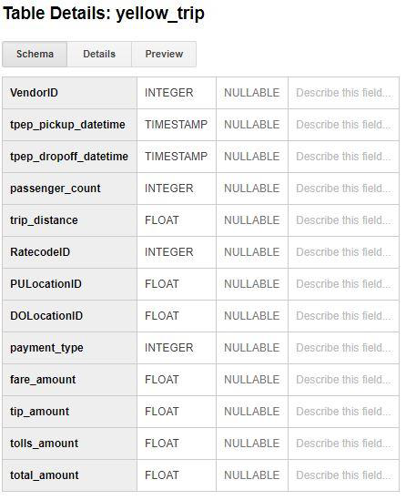
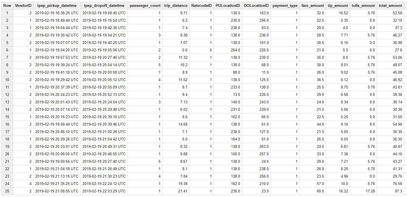
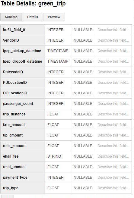
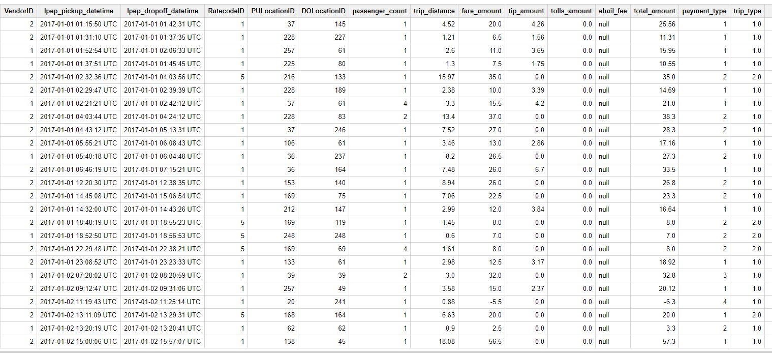
- In this project I have created the table for Green, Yellow, FHV taxis in Big Query as below
-
1. Yellow Taxis Table schema and content preview:
 2. Green Taxis Table schema and content preview:


Analytics
Graphical Analysis with the help of Google Data Studio
Analysis of Data
- After creating tables from the repository data, I selected a few columns on which I analyzed the data by querying and visualizing it. [chart 1] shows the most popular payment method for NYC taxies and the winner is a Credit card. This shows that people use cards mostly to pay for taxi fare. I have one observation, for 0.5% of trips mode of payment shows “No charges”. This can be due to multiple reasons so not really sure if that means ride was canceled or something else but I feel if data would have been more specific I could have projected more metrics on it.
- Let’s talk about [chart 2], which is talking about how many passengers are served by each taxi type. Looking at the data, it shows that Green taxi served very fewer customers compare to Yellow Taxi from 2017-2019. Yellow taxi is clearly a winner in this case by serving 250M+ customers. Please note that I found a few discrepancies in the data for 2019 for a yellow taxi so there may be some count issue for a yellow taxi but still it is clearly a winner in customer count.
- [chart 3] shows that no. of customers for a green taxi is kind of constant and there is no significant growth in ridership. Also, Yellow taxi data shows that growth in ridership is increasing and decreasing over the years over the month. This data can be better viewed if it is shown per year but I wanted to get an idea for the last 3 years aggregately so I calculated that way.
- In [chart 4] People say that nightlife is amazing in New York, I feel that my data is also proof of that. Looking at yellow taxi data, taxi is mostly busy between 1800 and 2000 hours. This is usually dinner time and after office hours. A green taxi is not really showing anything special, it looks like a taxi is busy throughout the day is same.
-
In [chart 5] and [chart 6], my motto for this chart was to check how generous people are towards taxis drives. I was looking for a specific pattern like is there a specific day or month when people are more generous in tips but after looking at the data I didn’t find such facts. Instead, I found that every year people have shown their generosity towards drives as there is no spike in the data graph and also tip amount has grown over the years. Also, it shows that tip amount is growing over the year for green taxies as well as yellow taxis, but the spike in the yellow taxis cab shows the data discrepancy which I found during loading data to Big Query.
- I found the two interesting facts while analyzing the data they are as below:
- Trends in Payment mode: Over the year “No charge” mode of payment is reduced for Green taxis[Table 1], but not the same case for yellow taxis[Table 2]. Also, there is only one electronic mode of payment available in NYC TLC, so there is a scope of development for NYC TLC cooperation as well as the fintech industry to include more electronic payment modes like e-wallets, apple pay, google pay etc.
- Busiest pick up location: Another interesting fact can help the department of transport to manage the traffic and parking problem as [Table 3] and [Table 4] shows which are the busiest pickup location ids for both the taxis.
- Trends in Payment mode: Over the year “No charge” mode of payment is reduced for Green taxis[Table 1], but not the same case for yellow taxis[Table 2]. Also, there is only one electronic mode of payment available in NYC TLC, so there is a scope of development for NYC TLC cooperation as well as the fintech industry to include more electronic payment modes like e-wallets, apple pay, google pay etc.
Challenges
- Skewed Data: I see that data for a yellow taxis for 2019 was not correct and it was showing data from 2018 and previous years which is incorrect so my analysis got impact due to that. Also, many fields were null which also disturbed the overall analysis.I overcame this by manually creating a schema for tables as well as dropping the rows and columns with the help of python script to reduce the impact of it on data analysis.
- In correct data types: In green taxi data, for 2019 vendor ids were of type integer but for 2018 and 2017 they were of type float so it didn’t allow me to merge the data into the same table. I had to implement a solution where I created the 2019 table as a separate table from other tables (2017 and 2018 got merged into one table) and got the aggregated data by joining these 2 tables.
- Missing field values: Data for a mode of the payment was inconsistent since for few payment modes I couldn’t find the data from 2017-2019. There might be a case that those modes may never be used but I felt they had little discrepancies. I had to merge such data into the category as “other” to minimize the impact on my analysis.
- Data Studio issue with Array Aggregator: Looks like Google data studio is not able to handle data which is aggregated by array aggregators so I had to put screenshots of the outcome into the charts instead of some fancy charts which could have been better in visualization.
Future Work
- With the given data I could analyze few good things like which taxi is popular among New Yorkers, a popular mode of payment, busiest hours for taxis, rider generosity, etc. This helps to get interesting info about taxies in Big Apple but given more data, I would have done a more detailed analysis.
- I would have loved to get more info on taxi driver ratings, instead of location id may be lat-long would have helped to get a better picture, mode of payments would have been better, incidence info like accidents, delay in the pickup, traffic rule violations, trips per driver, how long driver worked in a day.
Query Execution Details
Below is the execution details to retrive Table 1-2 and Table 3-4 data from Big Query.
- Table 1 [ Green Taxis]
- Table 2 [Yellow Taxis]
- Table 3 [Green Taxis]
- Table 4 [Yellow Taxis]
Why Big Query ?
There are many useful as well as optimization features which is provided by Big Query some those are below:
- Complex analysis can be done via SQL and user-defined functions (UDFs)
- BigQuery is suitable for calculating metrics/stats/aggregates over a large amount of data
- Faster and user-friendly web UI for querying and data loading.
- Multiple-way to load the data like Google cloud storage, local storage, other cloud storage.
- Easy to integrate with Google Data Studio to visualize the data.
- Stream-insert is available for receiving/ingesting live data into tables.